Deep Learning & Art: Neural Style Transfer

In this assignment, you will learn about Neural Style Transfer. This algorithm was created by Gatys et al. (2015).

In this assignment, you will:

Most of the algorithms you've studied optimize a cost function to get a set of parameter values. In Neural Style Transfer, you'll optimize a cost function to get pixel values!

Updates

If you were working on the notebook before this update...

List of updates

1 - Problem Statement

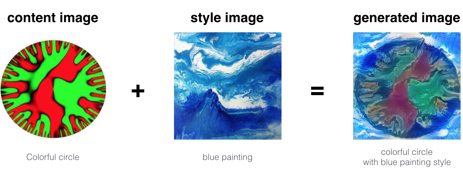
Neural Style Transfer (NST) is one of the most fun techniques in deep learning. As seen below, it merges two images, namely: a "content" image (C) and a "style" image (S), to create a "generated" image (G).

The generated image G combines the "content" of the image C with the "style" of image S.

In this example, you are going to generate an image of the Louvre museum in Paris (content image C), mixed with a painting by Claude Monet, a leader of the impressionist movement (style image S).

Let's see how you can do this.
2 - Transfer Learning

Neural Style Transfer (NST) uses a previously trained convolutional network, and builds on top of that. The idea of using a network trained on a different task and applying it to a new task is called transfer learning.

Following the original NST paper, we will use the VGG network. Specifically, we'll use VGG-19, a 19-layer version of the VGG network. This model has already been trained on the very large ImageNet database, and thus has learned to recognize a variety of low level features (at the shallower layers) and high level features (at the deeper layers).

Run the following code to load parameters from the VGG model. This may take a few seconds.

Assign input image to the model's input layer

To run an image through this network, you just have to feed the image to the model. In TensorFlow, you can do so using the tf.assign function. In particular, you will use the assign function like this:

model["input"].assign(image)

This assigns the image as an input to the model.

Activate a layer

After this, if you want to access the activations of a particular layer, say layer 4_2 when the network is run on this image, you would run a TensorFlow session on the correct tensor conv4_2, as follows:

sess.run(model["conv4_2"])

3 - Neural Style Transfer (NST)

We will build the Neural Style Transfer (NST) algorithm in three steps:

3.1 - Computing the content cost

In our running example, the content image C will be the picture of the Louvre Museum in Paris. Run the code below to see a picture of the Louvre.

The content image (C) shows the Louvre museum's pyramid surrounded by old Paris buildings, against a sunny sky with a few clouds.

3.1.1 - Make generated image G match the content of image C

Shallower versus deeper layers

Choose a "middle" activation layer $a^{[l]}$

We would like the "generated" image G to have similar content as the input image C. Suppose you have chosen some layer's activations to represent the content of an image.

Forward propagate image "C"

Forward propagate image "G"

Content Cost Function $J_{content}(C,G)$

We will define the content cost function as:

$$J_{content}(C,G) = \frac{1}{4 \times n_H \times n_W \times n_C}\sum _{ \text{all entries}} (a^{(C)} - a^{(G)})^2\tag{1} $$

Exercise: Compute the "content cost" using TensorFlow.

Instructions: The 3 steps to implement this function are:

  1. Retrieve dimensions from a_G:
    • To retrieve dimensions from a tensor X, use: X.get_shape().as_list()
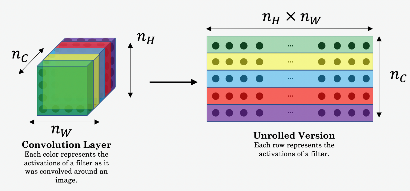
  2. Unroll a_C and a_G as explained in the picture above
  3. Compute the content cost:

Additional Hints for "Unrolling"

Expected Output:

**J_content** 6.76559

What you should remember

3.2 - Computing the style cost

For our running example, we will use the following style image:

This was painted in the style of impressionism.

Lets see how you can now define a "style" cost function $J_{style}(S,G)$.

3.2.1 - Style matrix

Gram matrix

Two meanings of the variable $G$

Compute $G_{gram}$

In Neural Style Transfer (NST), you can compute the Style matrix by multiplying the "unrolled" filter matrix with its transpose:

$$\mathbf{G}_{gram} = \mathbf{A}_{unrolled} \mathbf{A}_{unrolled}^T$$

$G_{(gram)i,j}$: correlation

The result is a matrix of dimension $(n_C,n_C)$ where $n_C$ is the number of filters (channels). The value $G_{(gram)i,j}$ measures how similar the activations of filter $i$ are to the activations of filter $j$.

$G_{(gram),i,i}$: prevalence of patterns or textures

By capturing the prevalence of different types of features ($G_{(gram)ii}$), as well as how much different features occur together ($G_{(gram)ij}$), the Style matrix $G_{gram}$ measures the style of an image.

Exercise:

Expected Output:

**GA** [[ 6.42230511 -4.42912197 -2.09668207]
[ -4.42912197 19.46583748 19.56387138]
[ -2.09668207 19.56387138 20.6864624 ]]

3.2.2 - Style cost

Your goal will be to minimize the distance between the Gram matrix of the "style" image S and the gram matrix of the "generated" image G.

$$J_{style}^{[l]}(S,G) = \frac{1}{4 \times {n_C}^2 \times (n_H \times n_W)^2} \sum _{i=1}^{n_C}\sum_{j=1}^{n_C}(G^{(S)}_{(gram)i,j} - G^{(G)}_{(gram)i,j})^2\tag{2} $$

Exercise: Compute the style cost for a single layer.

Instructions: The 3 steps to implement this function are:

  1. Retrieve dimensions from the hidden layer activations a_G:
    • To retrieve dimensions from a tensor X, use: X.get_shape().as_list()
  2. Unroll the hidden layer activations a_S and a_G into 2D matrices, as explained in the picture above (see the images in the sections "computing the content cost" and "style matrix").
  3. Compute the Style matrix of the images S and G. (Use the function you had previously written.)
  4. Compute the Style cost:

Additional Hints

Expected Output:

**J_style_layer** 9.19028

3.2.3 Style Weights

You can combine the style costs for different layers as follows:

$$J_{style}(S,G) = \sum_{l} \lambda^{[l]} J^{[l]}_{style}(S,G)$$

where the values for $\lambda^{[l]}$ are given in STYLE_LAYERS.

Exercise: compute style cost

Description of compute_style_cost

For each layer:

Once you're done with the loop:

Note: In the inner-loop of the for-loop above, a_G is a tensor and hasn't been evaluated yet. It will be evaluated and updated at each iteration when we run the TensorFlow graph in model_nn() below.

What you should remember

3.3 - Defining the total cost to optimize

Finally, let's create a cost function that minimizes both the style and the content cost. The formula is:

$$J(G) = \alpha J_{content}(C,G) + \beta J_{style}(S,G)$$

Exercise: Implement the total cost function which includes both the content cost and the style cost.

Expected Output:

**J** 35.34667875478276

What you should remember

4 - Solving the optimization problem

Finally, let's put everything together to implement Neural Style Transfer!

Here's what the program will have to do:

  1. Create an Interactive Session
  2. Load the content image
  3. Load the style image
  4. Randomly initialize the image to be generated
  5. Load the VGG19 model
  6. Build the TensorFlow graph:
    • Run the content image through the VGG19 model and compute the content cost
    • Run the style image through the VGG19 model and compute the style cost
    • Compute the total cost
    • Define the optimizer and the learning rate
  7. Initialize the TensorFlow graph and run it for a large number of iterations, updating the generated image at every step.

Lets go through the individual steps in detail.

Interactive Sessions

You've previously implemented the overall cost $J(G)$. We'll now set up TensorFlow to optimize this with respect to $G$.

Start the interactive session.

Content image

Let's load, reshape, and normalize our "content" image (the Louvre museum picture):

Style image

Let's load, reshape and normalize our "style" image (Claude Monet's painting):

Generated image correlated with content image

Now, we initialize the "generated" image as a noisy image created from the content_image.

Load pre-trained VGG19 model

Next, as explained in part (2), let's load the VGG19 model.

Content Cost

To get the program to compute the content cost, we will now assign a_C and a_G to be the appropriate hidden layer activations. We will use layer conv4_2 to compute the content cost. The code below does the following:

  1. Assign the content image to be the input to the VGG model.
  2. Set a_C to be the tensor giving the hidden layer activation for layer "conv4_2".
  3. Set a_G to be the tensor giving the hidden layer activation for the same layer.
  4. Compute the content cost using a_C and a_G.

Note: At this point, a_G is a tensor and hasn't been evaluated. It will be evaluated and updated at each iteration when we run the Tensorflow graph in model_nn() below.

Style cost

Exercise: total cost

Optimizer

Exercise: implement the model

Hints

Run the following cell to generate an artistic image. It should take about 3min on CPU for every 20 iterations but you start observing attractive results after ≈140 iterations. Neural Style Transfer is generally trained using GPUs.

Expected Output:

**Iteration 0 : ** total cost = 5.05035e+09
content cost = 7877.67
style cost = 1.26257e+08

You're done! After running this, in the upper bar of the notebook click on "File" and then "Open". Go to the "/output" directory to see all the saved images. Open "generated_image" to see the generated image! :)

You should see something the image presented below on the right:

We didn't want you to wait too long to see an initial result, and so had set the hyperparameters accordingly. To get the best looking results, running the optimization algorithm longer (and perhaps with a smaller learning rate) might work better. After completing and submitting this assignment, we encourage you to come back and play more with this notebook, and see if you can generate even better looking images.

Here are few other examples:

5 - Test with your own image (Optional/Ungraded)

Finally, you can also rerun the algorithm on your own images!

To do so, go back to part 4 and change the content image and style image with your own pictures. In detail, here's what you should do:

  1. Click on "File -> Open" in the upper tab of the notebook
  2. Go to "/images" and upload your images (requirement: (WIDTH = 300, HEIGHT = 225)), rename them "my_content.png" and "my_style.png" for example.
  3. Change the code in part (3.4) from :
    content_image = scipy.misc.imread("images/louvre.jpg")
    style_image = scipy.misc.imread("images/claude-monet.jpg")
    
    to:
    content_image = scipy.misc.imread("images/my_content.jpg")
    style_image = scipy.misc.imread("images/my_style.jpg")
    
  4. Rerun the cells (you may need to restart the Kernel in the upper tab of the notebook).

You can share your generated images with us on social media with the hashtag #deeplearniNgAI or by direct tagging!

You can also tune your hyperparameters:

6 - Conclusion

Great job on completing this assignment! You are now able to use Neural Style Transfer to generate artistic images. This is also your first time building a model in which the optimization algorithm updates the pixel values rather than the neural network's parameters. Deep learning has many different types of models and this is only one of them!

What you should remember

Congratulations on finishing the course!

This was the final programming exercise of this course. Congratulations--you've finished all the programming exercises of this course on Convolutional Networks! We hope to also see you in Course 5, on Sequence models!

References:

The Neural Style Transfer algorithm was due to Gatys et al. (2015). Harish Narayanan and Github user "log0" also have highly readable write-ups from which we drew inspiration. The pre-trained network used in this implementation is a VGG network, which is due to Simonyan and Zisserman (2015). Pre-trained weights were from the work of the MathConvNet team.