Welcome to Course 4's second assignment! In this notebook, you will:
After this assignment you will be able to:
We assume here that you are already familiar with TensorFlow. If you are not, please refer the TensorFlow Tutorial of the third week of Course 2 ("Improving deep neural networks").
initialize_parameters
: added details about tf.get_variable, eval
. Clarified test case.forward_propagation
: clarified instructions, use "F" to store "flatten" layer.In the previous assignment, you built helper functions using numpy to understand the mechanics behind convolutional neural networks. Most practical applications of deep learning today are built using programming frameworks, which have many built-in functions you can simply call.
As usual, we will start by loading in the packages.
import math
import numpy as np
import h5py
import matplotlib.pyplot as plt
import scipy
from PIL import Image
from scipy import ndimage
import tensorflow as tf
from tensorflow.python.framework import ops
from cnn_utils import *
%matplotlib inline
np.random.seed(1)
Run the next cell to load the "SIGNS" dataset you are going to use.
# Loading the data (signs)
X_train_orig, Y_train_orig, X_test_orig, Y_test_orig, classes = load_dataset()
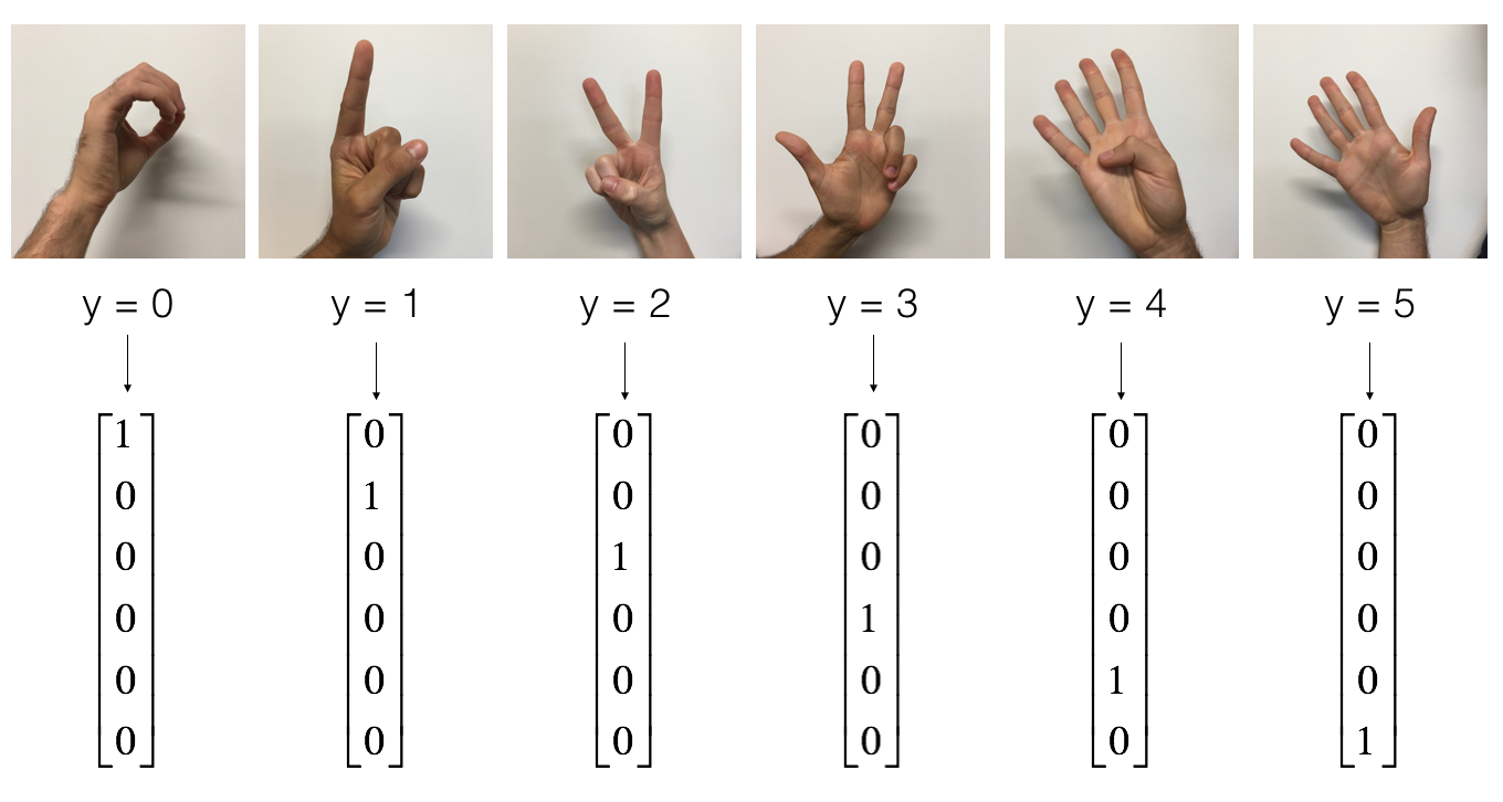
As a reminder, the SIGNS dataset is a collection of 6 signs representing numbers from 0 to 5.
The next cell will show you an example of a labelled image in the dataset. Feel free to change the value of index
below and re-run to see different examples.
# Example of a picture
index = 6
plt.imshow(X_train_orig[index])
print ("y = " + str(np.squeeze(Y_train_orig[:, index])))
y = 2
In Course 2, you had built a fully-connected network for this dataset. But since this is an image dataset, it is more natural to apply a ConvNet to it.
To get started, let's examine the shapes of your data.
X_train = X_train_orig/255.
X_test = X_test_orig/255.
Y_train = convert_to_one_hot(Y_train_orig, 6).T
Y_test = convert_to_one_hot(Y_test_orig, 6).T
print ("number of training examples = " + str(X_train.shape[0]))
print ("number of test examples = " + str(X_test.shape[0]))
print ("X_train shape: " + str(X_train.shape))
print ("Y_train shape: " + str(Y_train.shape))
print ("X_test shape: " + str(X_test.shape))
print ("Y_test shape: " + str(Y_test.shape))
conv_layers = {}
number of training examples = 1080 number of test examples = 120 X_train shape: (1080, 64, 64, 3) Y_train shape: (1080, 6) X_test shape: (120, 64, 64, 3) Y_test shape: (120, 6)
TensorFlow requires that you create placeholders for the input data that will be fed into the model when running the session.
Exercise: Implement the function below to create placeholders for the input image X and the output Y. You should not define the number of training examples for the moment. To do so, you could use "None" as the batch size, it will give you the flexibility to choose it later. Hence X should be of dimension [None, n_H0, n_W0, n_C0] and Y should be of dimension [None, n_y]. Hint: search for the tf.placeholder documentation".
# GRADED FUNCTION: create_placeholders
def create_placeholders(n_H0, n_W0, n_C0, n_y):
"""
Creates the placeholders for the tensorflow session.
Arguments:
n_H0 -- scalar, height of an input image
n_W0 -- scalar, width of an input image
n_C0 -- scalar, number of channels of the input
n_y -- scalar, number of classes
Returns:
X -- placeholder for the data input, of shape [None, n_H0, n_W0, n_C0] and dtype "float"
Y -- placeholder for the input labels, of shape [None, n_y] and dtype "float"
"""
### START CODE HERE ### (≈2 lines)
X = tf.placeholder(tf.float32, shape=((None, n_H0, n_W0, n_C0)))
Y = tf.placeholder(tf.float32, shape=((None, n_y)))
### END CODE HERE ###
return X, Y
X, Y = create_placeholders(64, 64, 3, 6)
print ("X = " + str(X))
print ("Y = " + str(Y))
X = Tensor("Placeholder:0", shape=(?, 64, 64, 3), dtype=float32) Y = Tensor("Placeholder_1:0", shape=(?, 6), dtype=float32)
Expected Output
X = Tensor("Placeholder:0", shape=(?, 64, 64, 3), dtype=float32) |
Y = Tensor("Placeholder_1:0", shape=(?, 6), dtype=float32) |
You will initialize weights/filters $W1$ and $W2$ using tf.contrib.layers.xavier_initializer(seed = 0)
. You don't need to worry about bias variables as you will soon see that TensorFlow functions take care of the bias. Note also that you will only initialize the weights/filters for the conv2d functions. TensorFlow initializes the layers for the fully connected part automatically. We will talk more about that later in this assignment.
Exercise: Implement initialize_parameters(). The dimensions for each group of filters are provided below. Reminder - to initialize a parameter $W$ of shape [1,2,3,4] in Tensorflow, use:
W = tf.get_variable("W", [1,2,3,4], initializer = ...)
Search for the tf.get_variable documentation. Notice that the documentation says:
Gets an existing variable with these parameters or create a new one.
So we can use this function to create a tensorflow variable with the specified name, but if the variables already exist, it will get the existing variable with that same name.
# GRADED FUNCTION: initialize_parameters
def initialize_parameters():
"""
Initializes weight parameters to build a neural network with tensorflow. The shapes are:
W1 : [4, 4, 3, 8]
W2 : [2, 2, 8, 16]
Note that we will hard code the shape values in the function to make the grading simpler.
Normally, functions should take values as inputs rather than hard coding.
Returns:
parameters -- a dictionary of tensors containing W1, W2
"""
tf.set_random_seed(1) # so that your "random" numbers match ours
### START CODE HERE ### (approx. 2 lines of code)
W1 = tf.get_variable("W1", [4, 4, 3, 8], initializer = tf.contrib.layers.xavier_initializer(seed = 0))
W2 = tf.get_variable("W2", [2, 2, 8, 16], initializer = tf.contrib.layers.xavier_initializer(seed = 0))
### END CODE HERE ###
parameters = {"W1": W1,
"W2": W2}
return parameters
tf.reset_default_graph()
with tf.Session() as sess_test:
parameters = initialize_parameters()
init = tf.global_variables_initializer()
sess_test.run(init)
print("W1[1,1,1] = \n" + str(parameters["W1"].eval()[1,1,1]))
print("W1.shape: " + str(parameters["W1"].shape))
print("\n")
print("W2[1,1,1] = \n" + str(parameters["W2"].eval()[1,1,1]))
print("W2.shape: " + str(parameters["W2"].shape))
W1[1,1,1] = [ 0.00131723 0.14176141 -0.04434952 0.09197326 0.14984085 -0.03514394 -0.06847463 0.05245192] W1.shape: (4, 4, 3, 8) W2[1,1,1] = [-0.08566415 0.17750949 0.11974221 0.16773748 -0.0830943 -0.08058 -0.00577033 -0.14643836 0.24162132 -0.05857408 -0.19055021 0.1345228 -0.22779644 -0.1601823 -0.16117483 -0.10286498] W2.shape: (2, 2, 8, 16)
Expected Output:
W1[1,1,1] =
[ 0.00131723 0.14176141 -0.04434952 0.09197326 0.14984085 -0.03514394
-0.06847463 0.05245192]
W1.shape: (4, 4, 3, 8)
W2[1,1,1] =
[-0.08566415 0.17750949 0.11974221 0.16773748 -0.0830943 -0.08058
-0.00577033 -0.14643836 0.24162132 -0.05857408 -0.19055021 0.1345228
-0.22779644 -0.1601823 -0.16117483 -0.10286498]
W2.shape: (2, 2, 8, 16)
In TensorFlow, there are built-in functions that implement the convolution steps for you.
tf.nn.conv2d(X,W, strides = [1,s,s,1], padding = 'SAME'): given an input $X$ and a group of filters $W$, this function convolves $W$'s filters on X. The third parameter ([1,s,s,1]) represents the strides for each dimension of the input (m, n_H_prev, n_W_prev, n_C_prev). Normally, you'll choose a stride of 1 for the number of examples (the first value) and for the channels (the fourth value), which is why we wrote the value as [1,s,s,1]
. You can read the full documentation on conv2d.
tf.nn.max_pool(A, ksize = [1,f,f,1], strides = [1,s,s,1], padding = 'SAME'): given an input A, this function uses a window of size (f, f) and strides of size (s, s) to carry out max pooling over each window. For max pooling, we usually operate on a single example at a time and a single channel at a time. So the first and fourth value in [1,f,f,1]
are both 1. You can read the full documentation on max_pool.
tf.nn.relu(Z): computes the elementwise ReLU of Z (which can be any shape). You can read the full documentation on relu.
tf.contrib.layers.flatten(P): given a tensor "P", this function takes each training (or test) example in the batch and flattens it into a 1D vector.
tf.contrib.layers.fully_connected(F, num_outputs): given the flattened input F, it returns the output computed using a fully connected layer. You can read the full documentation on full_connected.
In the last function above (tf.contrib.layers.fully_connected
), the fully connected layer automatically initializes weights in the graph and keeps on training them as you train the model. Hence, you did not need to initialize those weights when initializing the parameters.
The words "window", "kernel", and "filter" are used to refer to the same thing. This is why the parameter ksize
refers to "kernel size", and we use (f,f)
to refer to the filter size. Both "kernel" and "filter" refer to the "window."
Exercise
Implement the forward_propagation
function below to build the following model: CONV2D -> RELU -> MAXPOOL -> CONV2D -> RELU -> MAXPOOL -> FLATTEN -> FULLYCONNECTED
. You should use the functions above.
In detail, we will use the following parameters for all the steps:
# GRADED FUNCTION: forward_propagation
def forward_propagation(X, parameters):
"""
Implements the forward propagation for the model:
CONV2D -> RELU -> MAXPOOL -> CONV2D -> RELU -> MAXPOOL -> FLATTEN -> FULLYCONNECTED
Note that for simplicity and grading purposes, we'll hard-code some values
such as the stride and kernel (filter) sizes.
Normally, functions should take these values as function parameters.
Arguments:
X -- input dataset placeholder, of shape (input size, number of examples)
parameters -- python dictionary containing your parameters "W1", "W2"
the shapes are given in initialize_parameters
Returns:
Z3 -- the output of the last LINEAR unit
"""
# Retrieve the parameters from the dictionary "parameters"
W1 = parameters['W1']
W2 = parameters['W2']
### START CODE HERE ###
# CONV2D: stride of 1, padding 'SAME'
Z1 = tf.nn.conv2d(X,W1, strides = [1,1,1,1], padding = 'SAME')
# RELU
A1 = tf.nn.relu(Z1)
# MAXPOOL: window 8x8, stride 8, padding 'SAME'
P1 = tf.nn.max_pool(A1, ksize = [1,8,8,1], strides = [1,8,8,1], padding = 'SAME')
# CONV2D: filters W2, stride 1, padding 'SAME'
Z2 = tf.nn.conv2d(P1,W2, strides = [1,1,1,1], padding = 'SAME')
# RELU
A2 = tf.nn.relu(Z2)
# MAXPOOL: window 4x4, stride 4, padding 'SAME'
P2 = tf.nn.max_pool(A2, ksize = [1,4,4,1], strides = [1,4,4,1], padding = 'SAME')
# FLATTEN
F = tf.contrib.layers.flatten(P2)
# FULLY-CONNECTED without non-linear activation function (not not call softmax).
# 6 neurons in output layer. Hint: one of the arguments should be "activation_fn=None"
Z3 = tf.contrib.layers.fully_connected(F, 6, activation_fn=None)
### END CODE HERE ###
return Z3
tf.reset_default_graph()
with tf.Session() as sess:
np.random.seed(1)
X, Y = create_placeholders(64, 64, 3, 6)
parameters = initialize_parameters()
Z3 = forward_propagation(X, parameters)
init = tf.global_variables_initializer()
sess.run(init)
a = sess.run(Z3, {X: np.random.randn(2,64,64,3), Y: np.random.randn(2,6)})
print("Z3 = \n" + str(a))
Z3 = [[-0.44670227 -1.57208765 -1.53049231 -2.31013036 -1.29104376 0.46852064] [-0.17601591 -1.57972014 -1.4737016 -2.61672091 -1.00810647 0.5747785 ]]
Expected Output:
Z3 =
[[-0.44670227 -1.57208765 -1.53049231 -2.31013036 -1.29104376 0.46852064]
[-0.17601591 -1.57972014 -1.4737016 -2.61672091 -1.00810647 0.5747785 ]]
Implement the compute cost function below. Remember that the cost function helps the neural network see how much the model's predictions differ from the correct labels. By adjusting the weights of the network to reduce the cost, the neural network can improve its predictions.
You might find these two functions helpful:
softmax_cross_entropy_with_logits
takes logits as input (and not activations); then uses the model to predict using softmax, and then compares the predictions with the true labels using cross entropy. These are done with a single function to optimize the calculations.Exercise: Compute the cost below using the function above.
# GRADED FUNCTION: compute_cost
def compute_cost(Z3, Y):
"""
Computes the cost
Arguments:
Z3 -- output of forward propagation (output of the last LINEAR unit), of shape (number of examples, 6)
Y -- "true" labels vector placeholder, same shape as Z3
Returns:
cost - Tensor of the cost function
"""
### START CODE HERE ### (1 line of code)
cost = tf.reduce_mean(tf.nn.softmax_cross_entropy_with_logits(logits = Z3, labels = Y))
### END CODE HERE ###
return cost
tf.reset_default_graph()
with tf.Session() as sess:
np.random.seed(1)
X, Y = create_placeholders(64, 64, 3, 6)
parameters = initialize_parameters()
Z3 = forward_propagation(X, parameters)
cost = compute_cost(Z3, Y)
init = tf.global_variables_initializer()
sess.run(init)
a = sess.run(cost, {X: np.random.randn(4,64,64,3), Y: np.random.randn(4,6)})
print("cost = " + str(a))
cost = 2.91034
Expected Output:
cost = 2.91034
Finally you will merge the helper functions you implemented above to build a model. You will train it on the SIGNS dataset.
Exercise: Complete the function below.
The model below should:
Finally you will create a session and run a for loop for num_epochs, get the mini-batches, and then for each mini-batch you will optimize the function. Hint for initializing the variables
You can use tf.train.AdamOptimizer(learning_rate = ...)
to create the optimizer. The optimizer has a minimize(loss=...)
function that you'll call to set the cost function that the optimizer will minimize.
For details, check out the documentation for Adam Optimizer
If you took course 2 of the deep learning specialization, you implemented random_mini_batches()
in the "Optimization" programming assignment. This function returns a list of mini-batches. It is already implemented in the cnn_utils.py
file and imported here, so you can call it like this:
minibatches = random_mini_batches(X, Y, mini_batch_size = 64, seed = 0)
(You will want to choose the correct variable names when you use it in your code).
Within a loop, for each mini-batch, you'll use the tf.Session
object (named sess
) to feed a mini-batch of inputs and labels into the neural network and evaluate the tensors for the optimizer as well as the cost. Remember that we built a graph data structure and need to feed it inputs and labels and use sess.run()
in order to get values for the optimizer and cost.
You'll use this kind of syntax:
output_for_var1, output_for_var2 = sess.run(
fetches=[var1, var2],
feed_dict={var_inputs: the_batch_of_inputs,
var_labels: the_batch_of_labels}
)
sess.run
takes its first argument fetches
as a list of objects that you want it to evaluate (in this case, we want to evaluate the optimizer and the cost). feed_dict
parameter. tf.placeholder
variables that we created in the create_placeholders
function above. fetches
. For more information on how to use sess.run, see the documentation tf.Sesssion#run documentation.
# GRADED FUNCTION: model
def model(X_train, Y_train, X_test, Y_test, learning_rate = 0.009,
num_epochs = 100, minibatch_size = 64, print_cost = True):
"""
Implements a three-layer ConvNet in Tensorflow:
CONV2D -> RELU -> MAXPOOL -> CONV2D -> RELU -> MAXPOOL -> FLATTEN -> FULLYCONNECTED
Arguments:
X_train -- training set, of shape (None, 64, 64, 3)
Y_train -- test set, of shape (None, n_y = 6)
X_test -- training set, of shape (None, 64, 64, 3)
Y_test -- test set, of shape (None, n_y = 6)
learning_rate -- learning rate of the optimization
num_epochs -- number of epochs of the optimization loop
minibatch_size -- size of a minibatch
print_cost -- True to print the cost every 100 epochs
Returns:
train_accuracy -- real number, accuracy on the train set (X_train)
test_accuracy -- real number, testing accuracy on the test set (X_test)
parameters -- parameters learnt by the model. They can then be used to predict.
"""
ops.reset_default_graph() # to be able to rerun the model without overwriting tf variables
tf.set_random_seed(1) # to keep results consistent (tensorflow seed)
seed = 3 # to keep results consistent (numpy seed)
(m, n_H0, n_W0, n_C0) = X_train.shape
n_y = Y_train.shape[1]
costs = [] # To keep track of the cost
# Create Placeholders of the correct shape
### START CODE HERE ### (1 line)
X, Y = create_placeholders(n_H0, n_W0, n_C0, n_y)
### END CODE HERE ###
# Initialize parameters
### START CODE HERE ### (1 line)
parameters = initialize_parameters()
### END CODE HERE ###
# Forward propagation: Build the forward propagation in the tensorflow graph
### START CODE HERE ### (1 line)
Z3 = forward_propagation(X, parameters)
### END CODE HERE ###
# Cost function: Add cost function to tensorflow graph
### START CODE HERE ### (1 line)
cost = compute_cost(Z3, Y)
### END CODE HERE ###
# Backpropagation: Define the tensorflow optimizer. Use an AdamOptimizer that minimizes the cost.
### START CODE HERE ### (1 line)
optimizer = tf.train.AdamOptimizer(learning_rate).minimize(cost)
### END CODE HERE ###
# Initialize all the variables globally
init = tf.global_variables_initializer()
# Start the session to compute the tensorflow graph
with tf.Session() as sess:
# Run the initialization
sess.run(init)
# Do the training loop
for epoch in range(num_epochs):
minibatch_cost = 0.
num_minibatches = int(m / minibatch_size) # number of minibatches of size minibatch_size in the train set
seed = seed + 1
minibatches = random_mini_batches(X_train, Y_train, minibatch_size, seed)
for minibatch in minibatches:
# Select a minibatch
(minibatch_X, minibatch_Y) = minibatch
"""
# IMPORTANT: The line that runs the graph on a minibatch.
# Run the session to execute the optimizer and the cost.
# The feedict should contain a minibatch for (X,Y).
"""
### START CODE HERE ### (1 line)
_ , temp_cost = sess.run([optimizer, cost], feed_dict={X: minibatch_X , Y: minibatch_Y})
### END CODE HERE ###
minibatch_cost += temp_cost / num_minibatches
# Print the cost every epoch
if print_cost == True and epoch % 5 == 0:
print ("Cost after epoch %i: %f" % (epoch, minibatch_cost))
if print_cost == True and epoch % 1 == 0:
costs.append(minibatch_cost)
# plot the cost
plt.plot(np.squeeze(costs))
plt.ylabel('cost')
plt.xlabel('iterations (per tens)')
plt.title("Learning rate =" + str(learning_rate))
plt.show()
# Calculate the correct predictions
predict_op = tf.argmax(Z3, 1)
correct_prediction = tf.equal(predict_op, tf.argmax(Y, 1))
# Calculate accuracy on the test set
accuracy = tf.reduce_mean(tf.cast(correct_prediction, "float"))
print(accuracy)
train_accuracy = accuracy.eval({X: X_train, Y: Y_train})
test_accuracy = accuracy.eval({X: X_test, Y: Y_test})
print("Train Accuracy:", train_accuracy)
print("Test Accuracy:", test_accuracy)
return train_accuracy, test_accuracy, parameters
Run the following cell to train your model for 100 epochs. Check if your cost after epoch 0 and 5 matches our output. If not, stop the cell and go back to your code!
_, _, parameters = model(X_train, Y_train, X_test, Y_test)
Cost after epoch 0: 1.917929 Cost after epoch 5: 1.506757 Cost after epoch 10: 0.955359 Cost after epoch 15: 0.845802 Cost after epoch 20: 0.701174 Cost after epoch 25: 0.571977 Cost after epoch 30: 0.518435 Cost after epoch 35: 0.495806 Cost after epoch 40: 0.429827 Cost after epoch 45: 0.407291 Cost after epoch 50: 0.366394 Cost after epoch 55: 0.376922 Cost after epoch 60: 0.299491 Cost after epoch 65: 0.338870 Cost after epoch 70: 0.316400 Cost after epoch 75: 0.310413 Cost after epoch 80: 0.249549 Cost after epoch 85: 0.243457 Cost after epoch 90: 0.200031 Cost after epoch 95: 0.175452
Tensor("Mean_1:0", shape=(), dtype=float32) Train Accuracy: 0.940741 Test Accuracy: 0.783333
Expected output: although it may not match perfectly, your expected output should be close to ours and your cost value should decrease.
**Cost after epoch 0 =** | 1.917929 |
**Cost after epoch 5 =** | 1.506757 |
**Train Accuracy =** | 0.940741 |
**Test Accuracy =** | 0.783333 |
Congratulations! You have finished the assignment and built a model that recognizes SIGN language with almost 80% accuracy on the test set. If you wish, feel free to play around with this dataset further. You can actually improve its accuracy by spending more time tuning the hyperparameters, or using regularization (as this model clearly has a high variance).
Once again, here's a thumbs up for your work!
fname = "images/thumbs_up.jpg"
image = np.array(ndimage.imread(fname, flatten=False))
my_image = scipy.misc.imresize(image, size=(64,64))
plt.imshow(my_image)
<matplotlib.image.AxesImage at 0x7f641dc44748>